A Transformer and a Mamba model have almost nothing in common. Different math, different inductive biases, different assumptions about what makes a sequence learnable. Train them on the same task and they develop completely different internal strategies. But in my experiment, they agreed on one thing: where to stop. Same ceiling, same number, arrived at from opposite directions. When two models that share nothing agree on a limit, the limit is probably not in the models.
The experiment
I was working on a binary classification task over long sequences. The event-stream data is roughly 4,000 tokens per example. We sized it that way so a full training run fits under an hour on a consumer GPU on RunPod. My intuition is that the signal is sparsely distributed across the sequence. This is the kind of problem where the answer depends on patterns in the history, not just the most recent observation. The implementation was done by AI agents (Claude and Codex) under my direction. We trained two architectures on the same data: a Transformer and a Mamba model. I chose these two because in earlier local testing at shorter sequences (256 tokens), the Transformer actually beat Mamba. The reversal happened when we moved to 4,000 tokens on the cloud. Something about long-sequence processing specifically broke the Transformer, and I wanted to understand what.
These are fundamentally different machines. Transformers famously compute pairwise attention between every token in the sequence. Each position looks at every other position to decide what matters. Mamba is a state-space model that scans through the sequence one step at a time, selectively gating what to remember and what to forget. No pairwise computation, no quadratic scaling. Different inductive biases, different assumptions about what makes a sequence learnable.
Both models were small (~115K parameters), trained on the same hardware, same data, same sequence lengths. A controlled comparison.
What actually happened
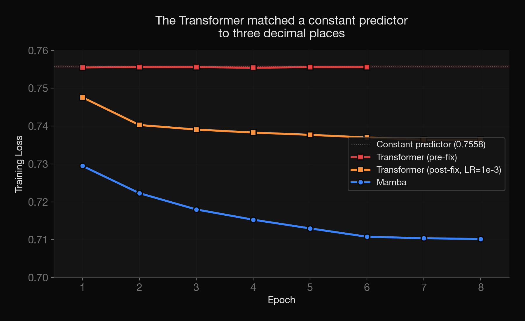
Initially, the transformer didn’t learn anything at all. Its training loss settled at 0.7555. For context, a model that predicts the same constant for every input, ignoring the data entirely, would achieve a loss of 0.7558 given this distribution. And the Transformer matched this degenerate case almost exactly across three full epochs. It was producing non-discriminative outputs. Each epoch also introduced random additional features into the same examples, so the model was seeing different slices of the input across epochs. It wasn’t starved for variety. So this was puzzling.
Mamba’s loss started below that baseline from the first epoch and kept declining. So this was learning something.
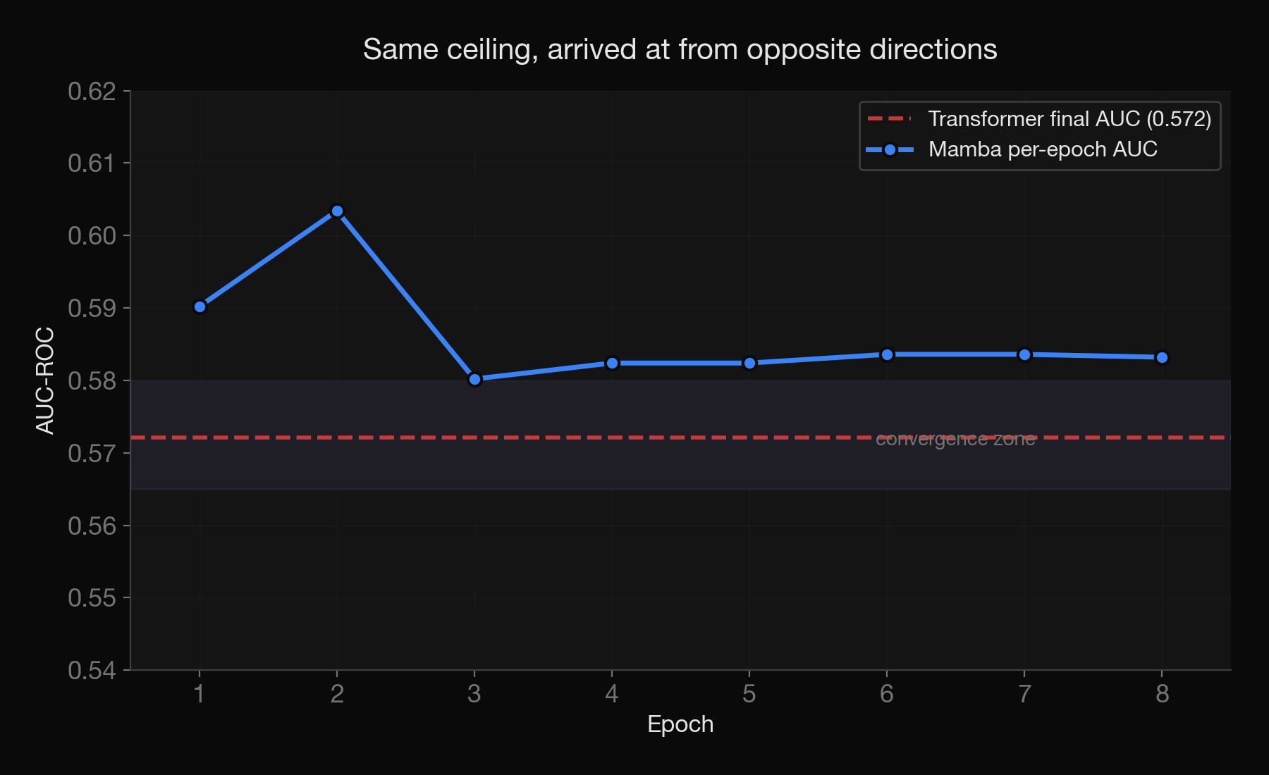
Why did the Transformer fail? My explanation is a conjecture, I didn’t measure gradient norms per layer. It was most likely because of gradient dilution through softmax: at 4,096 positions, initial attention weight per position is roughly 1/4096, and gradient scaling goes as p(1-p), which at p ≈ 0.00024 is vanishingly small. When tasked with identifying potential solutions Codex and Claude working together found that existing benchmarks already should have told us to expect this. Specifically Long Range Arena benchmarks show: ((Tay et al., “Long Range Arena: A Benchmark for Efficient Transformers,” ICLR 2021.)) vanilla Transformers score 50-57% on the hardest long-sequence tasks while state-space models hit 86-96%. Codex and Claude acting as applied scientists came up with standard architectural fixes: larger head dimension, RoPE positional encoding, ((Su et al., “RoFormer: Enhanced Transformer with Rotary Position Embedding,” 2021.)) mean pooling. They recommended rigorous hypothesis testing. But GPU time is hard to come by, so I did a yolo run combining all the recommendations. The Transformer briefly flickered to an AUC of 0.604 at epoch 1, then collapsed to 0.500 by epoch 2. None of the fixes produced stable learning.
Now I could accept that the transformer had nothing to learn from (input representation has no signal). But that seemed dubious to me as I could already see mamba was learning. My suspicion was on the learning rate. The brief flicker suggested there was a local minima somewhere but it wasn’t stable. I then got Codex to run a hyperparameter sweep on a smaller shard first. It found a narrow window that worked (learning rate of exactly 1e-3; 2e-3 already degraded significantly). With this learning rate, the transformer did learn on full run.
Finally I had Mamba and Transformer both learning from the data. But weirdly, they both converged to the same plateau AUC of almost exactly 0.572. First entry in the ledger: two completely different architectures, same ceiling.
Btw, I didn’t design these experiments. At every turn I was asking the questions and verifying claims made by Claude and Codex. I was treating them as my applied scientist and a peer scientist who does peer review. My questions would be along the lines of: a/ what’s the latest research on small models training long sequences? b/ what hyperparameters they used and why? c/ should we be using flash attention? Is it actually being used in the training run. d/ what are the mechanistic interpretability technique that applies to this model? e/ Why wouldn’t we do linear probes? Simple things like that. The agents would then answer the questions, design experiments, take my feedback, and run the experiments. It was fascinating to see how far these models have come!
Weird result
Two architectures with entirely different mechanisms for processing sequences arrived at the same performance ceiling — this was weird. This suggested that my input feature engineering was beginning to hit a plateau rather than model architecture.
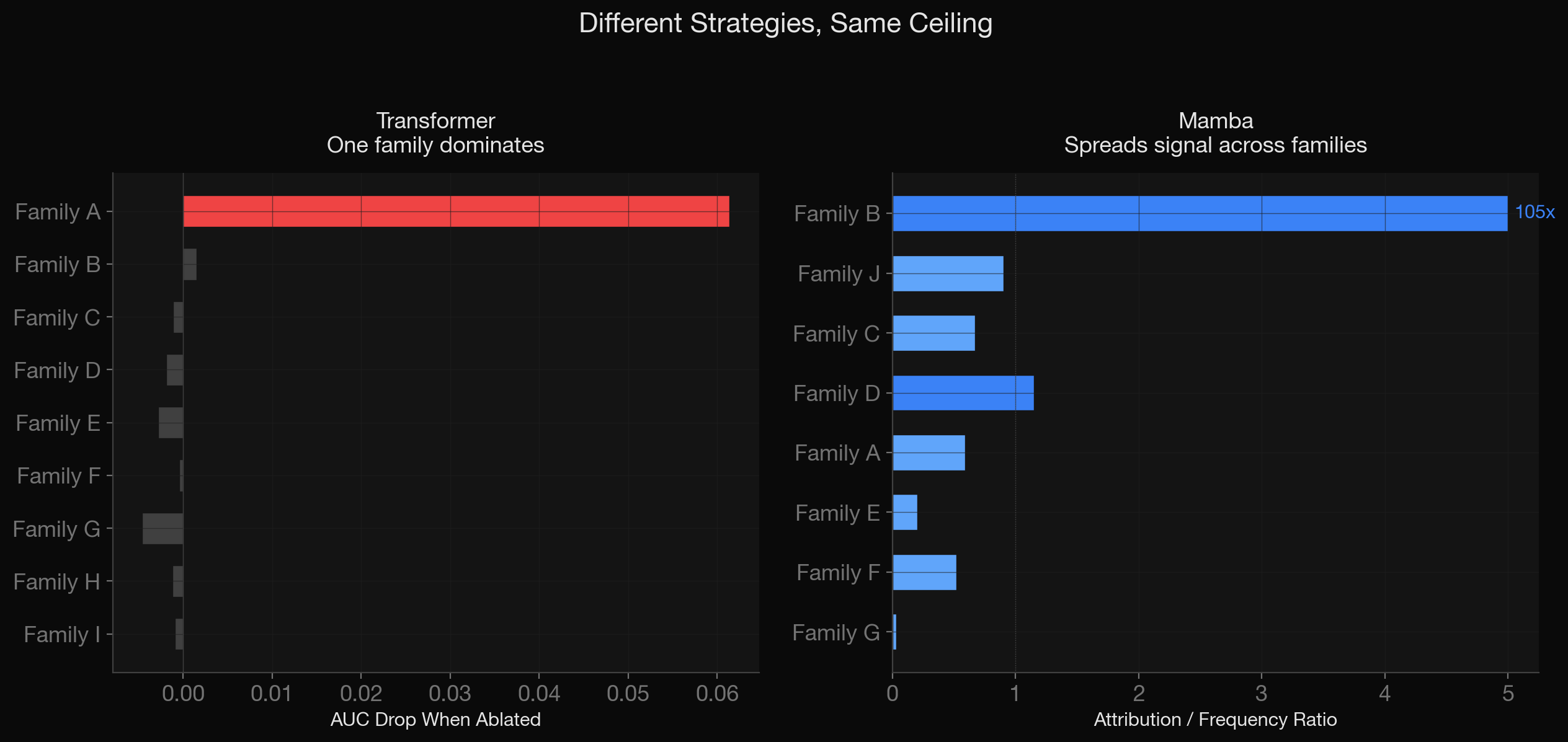
So the next step obviously was to look inside the box: mechanistic interpretability. Mamba and the Transformer developed completely different internal strategies. Mamba heavily processes structural tokens at the intake layer (high gating values, lots of internal computation) then discards those same tokens at decision time (0.20x their expected attribution) and relies on a different token family entirely for the classification signal. When we ablated the 14 input features that frame each prediction window, all 14 mattered nearly equally, within 0.0006 AUC of each other. This model was squeezing every feature it had.
The Transformer’s strategy was almost the opposite. It fixated on a single token family (0.061 AUC drop on ablation; every other family below 0.003). When we reversed the sequence order (fed the entire history backwards) predictions correlated with the originals at r = 0.981. It was treating a sequence problem as a bag-of-tokens problem. The positional encoding was doing effectively nothing.
Two additional observations reinforced my intuition that the representation was tapped out. First, hidden-state probes in both models performed below the majority-class baseline. This means the concepts the probes were trying to decode weren’t linearly accessible in hidden representations. Neither architecture was building rich compositional representations. Second, deeper layers in both models added minimal causal value on ablation (max AUC drop: 0.008 for any single layer). In other words, delete random layers, and the result doesn’t move all that much. Together, this evidence was enough to convince me that both models had already extracted what the representation could give them. More depth didn’t help.
In summary, the 14 features that define each prediction window appear to max out at roughly 0.57 AUC for binary classification on this task. More training doesn’t break through. 8 full epochs gained only +0.0015 AUC after the first half-epoch. A different architecture doesn’t break through. The mechanistic interpretability confirms that the model is using every feature available to it and not finding hidden combinatorial structure. The hand-engineered representation is tapped out. Second entry in the ledger.
Third entry, and this is the one I’m still sitting with: if two architectures and more training all converge on the same number, the path forward isn’t through the model. It’s through the data.
So what’s left
Feature engineering is not tapped out, at least not fully. The model squeezed everything out of the current 14 features, but that doesn’t mean better features can’t push the ceiling higher. Rich Sutton’s bitter lesson says ((Sutton, “The Bitter Lesson,” 2019.)) methods that scale with computation tend to win over methods that rely on human-engineered knowledge. If you have enough data, you can throw it at a model and it will figure it out.
But there is a parallel path: what do you do when you don’t have enough data? My experiment is sitting squarely in that zone. The ceiling at 0.57 AUC is not a model problem. It’s a data problem. And that opens up three loops, each more ambitious than the last.
The first loop is the one I’m running right now: improve the representation, re-train the models, run interpretability, learn what the model uses and what it ignores, improve the representation again. A newer feature set is already heading to RunPod for testing as I write this. This loop is feeble-human (yours truly) directed. I decide what features to try based on what the interpretability reveals. It works, but it depends on me asking the right questions. And it’s fighting the bitter lesson in some sense, keeping ‘me’ relevant, a ‘god of gaps’ as AGI closes in.
The second loop removes me from it. Get the agents (Claude, Codex) to run the first loop autonomously. They design the features, train the model, interpret the results, and iterate without my input. This is the bitter lesson applied at the agent level: scale the search with computation rather than relying on my intuition about what features matter. The ralph wiggum loop and Andrej Karpathy’s auto-research are templates here. Nothing too wild, but building the verifier so agents can’t cheat and coaxing them to be creative so they don’t repeat dull experiments is an interesting challenge.
The third loop is the one I keep coming back to. Instead of using the existing data at all, build a simulator that generates the inputs and outputs from scratch. A gym where the model trains against a synthetic environment with a built-in verifier. Many problems have the characteristic that solutions are hard to generate but easy to verify. If you can build the verifier, you can build a training loop around it. But building the verifier means defining the problem precisely enough that a machine can judge correctness. I don’t have this yet. It’s why asking the right question is harder than answering it once posed.
Two models that share nothing agreed on where to stop. But they also pointed me the way out of there!